
An Investigation into the Relationship Between
The Solar Activity Indices and Surface Climate
=============================================
The potential relationship between Solar activity – incoming solar radiation in all of its various forms – and surface climate, has already been discussed (see: Interesting Articles: Solar Variability) and it does seem that there is some anecdotal evidence to support the concept. To develop the idea further we need to examine, in depth, the charts and records to assess whether any hard evidence exists of an identifiable climatic reaction associated with a recorded variation in solar induced geomagnetic activity.
The particular weather phenomena under examination and discussion are associated with the ‘European Heat Wave 2003’, plus the severe winters experienced in Europe between 2009 and 2012 and the relationship between those events and recorded solar activity.
If we look for a cross reference between the recorded events in which we are interested and Sunspot Number records, we can find little that would support the idea of such a relationship. The heat wave occurred during the declining phase of a solar maximum, the cold during the ascent out of solar minimum, both periods being unremarkable in their activity levels. However, as we have already said, the existence of a sunspot does not imply the existence of a CME, much less a terrestrial impact – nor, indeed, does the absence of spots imply the absence of incoming material and it is becoming increasingly clear that solar wind and allied impacts have a significant effect on the behaviour of the atmosphere – we need, therefore, to look more closely at other solar behaviour.

If, then, we turn our attention to the ‘Solar Ap Progression’ records (see: ‘The Kp and Ap Indices’) we find that there is a somewhat startling cross correlation. A sharp spike is recorded occurring 2003 and a consecutive series of sharp dips December 2009/10/11 and 12. Indeed, if we examine in detail the Ap index for Carrington Rotations CR2104 / CR2105, for example, and others around the winter periods in question (http://eng.sepc.ac.cn/ApIndex.php ) we find that it is persistently inactive throughout with just a few isolated peaks reaching Ap10-15 and with Ap1-3 being common.![solar-cycle-planetary-a-index[1].gif](https://howtheatmosphereworks.wordpress.com/wp-content/uploads/2017/03/solar-cycle-planetary-a-index1.gif?w=786&h=601)
(Spörer’s Law Years)
The actual impact on the atmospheric structure may be viewed in the meteorological charts from the time, reproduced below. (see ‘Meteorological Chart Evaluation’)
It is relevant to note that the end of 2008 represented the deepest part of the sunspot null, yet it wasn’t until the Ap cycle plunged to its lowest levels in the years following that the extreme winters were experienced. As the charts show, in 2008 the cold was well advanced but did not reach the levels experienced later. This observation is consistent with the concept that a dip in solar impacts occurs coincident with the ‘leading edge’ years of each sunspot cycle (Spörer’s Law), and has a consequential effect upon surface climate. (Refer: “Ap Index Historical Analysis”)
An up-to-the-minute measurement of the ‘K’ index may be found here – http://www.swpc.noaa.gov/products/planetary-k-index – forecasts for Ap activity may be found here – http://eng.sepc.ac.cn/ApForecast.php – and details of current solar activity here – http://www.n3kl.org/sun/noaa.html – . A description of Spörer’s Law may be found here – https://en.wikipedia.org/wiki/Spörer’s_law -.
From these an assessment of the interrelationship between solar activity and observed climate response can be estimated, it should, however, be remembered that a short term ‘spike’ may not appear in the longer term records when the ‘Monthly’ or ‘Smoothed’ values are recorded although there may be some correspondingly short term reaction from the atmosphere itself.
The actual ‘Super Spike’ appearing on the chart in 2003 was associated with what became known as the ‘Halloween Super Storm’ when measurements went ‘off the scale’; of far greater interest to us is the general surge in broader based activity in the months preceding.
To understand the general atmospheric response we need to examine the statistics for Carrington Rotations CR2000 to CR2008, which data reveals substantial storming, reaching as much as Ap86 on 2003-08-18 with solar wind speeds reaching exceptional levels as high as 980 during that summer’s months originating from Coronal Holes CH42 to CH49. ( http://www.solen.info/solar/coronal_holes.html : refers)
The ‘super’ peak, on 2003-10-29 (CR2009), is recorded as Ap189, which may be compared to 2017 (daily, rather than the monthly averaged) figures of Ap40-50 at peak with Ap1-5 being average. However, as we have said, short term or extreme peaks may not be visibly recorded when smoothed averages are displayed.

We can extend our understanding of the relationship between solar activity and atmospheric response by examining the ‘Thermosphere Climate Index’. The unusually low levels achieved in 2008/2010 are clearly evident. Discussion paper can be viewed at- https://www.sciencedirect.com/science/article/pii/S1364682618301354?via%3Dihub
On that basis we can see that the low of 2008/10 is both deeper and wider than the previous low of spring 1954, the latter can be seen to have resulted in some serious, although short lived, cold over UK and Europe in the chart for 1st march of that year.

Ap Index  TCI Index
We can then assess the interrelationship between Ap Index and Thermosphere Index by displaying the two graphs on a comparable scale, as above. In doing this, we can confirm that the principle influence in TCI behaviour is “Ap” impact, it immediately becomes clear that a burst of Solar activity is very quickly followed by an increase in TCI and a decrease by a decline in TCI. The ‘Lag’ between impact and response may be estimated from comparison of the two graphs. This lag being dependant on the severity and degree of the change in the solar input. On average it seems that there is approximately one month delay between “Ap” impact and “TCI” thermal response.
Overall, the TCI follows the general trend of the Sunspot Number but is modulated by ‘Ap’ index impacts.
The potential for further deepening on the basis of the ‘Step Change’ discussed in ‘Ap Index Historical Analysis’ must be considered likely. Assessing the midpoint of solar cycles 19 to 23 it must be considered as being around the ‘Neutral’ mark. That for the 1970’s ‘Cooling Period’ would be ‘Cool’. That for cycle 24 appears to be very close to ‘Cold’, implying that the bottom of the coming trough could be unprecedentedly deep.
We need then, to establish whether simple but powerful solar wind, as distinct from the impact of a CME blast, can in fact inject significant amounts of energy into the Earthly environment. We can assess this most easily by measuring the Earth’s magnetic field and possible ground currents resulting from the incoming solar wind energy impact.

The above measurements show the result of solar wind impact emanating from a large, earth-facing, coronal hole occurring at a time when sunspot activity was minimal (small single, very simple, spot) and spot related Coronal mass ejections completely absent.

During the period April 21st to 25th, 2017, we had the opportunity to directly compare the impact of a CME glancing blow, and that of the solar wind from a coronal hole. Both impacts show similar amplitudes but the solar wind is significantly more prolonged.
Such activity implies that a significant response may be expected from solar wind disturbances, within the upper atmosphere, in the form of energy induced pressure and thermal variations with a resultant ‘tidal’ movement likely at lower levels.
Meteorological Chart Evaluation
To develop the idea further and assess whether there was a real, identifiable reaction in surface weather patterns, rather than simply a random variation, we can inspect the recorded atmosphere charts for those points in time that we have been considering and compare them with similar charts for the same point in time for other years around the same period.
Examining, firstly, the noted cold winter periods, we can use 2007 and 2008 as our control group where we find that on the Ap chart there was no serious dip recorded, in fact figures for the time were rather average. Examining then the deep atmosphere charts for those years we find that they also show average winter conditions.
2007….
2008 ….
When, however, we examine the atmosphere charts for the years 2009/10/11/12 we find a sharply defined ‘Plume’ of cold descending to cover the whole of Europe. This abnormally intense plume did not reappear in later years when the Ap down-spike was absent and winter conditions returned to what may be deemed to be Western European normal.
2009 ….
2010 ….
2011 ….

2012 ….
If we now turn our attention to the summer heat wave of 2003 we can use the years either side as a control group and compare with the record for 2003.
2002 and 2004/5 display conditions which may be described as ‘average’ over Europe for that time of the year, while 2003 displays a plume of abnormally high temperatures and an exaggerated northward distortion of the upper level isobars. This is most clearly seen in the northward distortion of the 600mb isobar, which line would rarely achieve latitudes beyond the North African coast but which is seen to reach southern UK in a significant northward distortion in this instance.
Using this concept and cross-referring to atmospheric charts we can often identify a similar response and relationship at other points in time.
2002 ….
2003… The heat wave…

2004 ….
2005 ….
It would seem unreasonable to assume that the injection of energy from Ap influences – or the lack of such energy in the case of a down-spike – would be sufficient, of itself, to distort the upper atmosphere profiles in the manner observed. What we can say is that it appears that pre-existing normal profiles and even specific weather events are exacerbated, expanded, even intensified, by the influence of externally originating geomagnetic activity, especially if that activity is prolonged or repetitive.
This response may be viewed as similar in nature to the activity of ocean tides, where a very slight change in gravity causes a slight bulge in the ocean but often massive tidal response at sensitive coastal areas; so the incoming solar energy causes a slight bulge in the upper atmosphere, resulting in significant movement at sensitive points in the atmospheric profile, with the consequent response in surface level weather patterns.
It is relevant to note that Geomagnetic activity tends to be lower around times of the Solstice and peaks at times of the Equinox. The reason for this is related to the seasonal orientation of Earth within the sun’s magnetic field–a phenomenon known as the “Russell-McPherron effect,” named after the researchers who first studied and explained it .
An interesting article can be found here …
http://www-ssc.igpp.ucla.edu/personnel/russell/papers/40/
Consequently, if activity is generally low at any given time, then it will fall to very low levels during the winter months giving an increased possibility of unusually severe winter weather, as has been noted in the years we have considered.

This tendency has been known for some time but not fully understood. NASA’s launch of the THEMIS satellites which, in 2007, detected magnetic ‘Ropes’ connecting Earth’s upper atmosphere directly to the Sun, thereby providing a pathway for solar wind to inject energy into the terrestrial atmosphere and the geomagnetic environment. The magnetic interconnection is at its lowest when the Earth’s magnetic field is at aligned to the solar plane and the heliospheric sheet. A detailed explanation of the geomagnetic ‘Rope’ theory may be obtained here …..
http://onlinelibrary.wiley.com/doi/10.1029/2007GL032933/full
Conditions which may be described as ‘Normal’ would be expected to display the usual variation between continental land mass and oceanic areas such that in summer the oceans would be cool, the land mass warm with the reverse being the case in winter. Upper level profiles tend to follow this variation giving rise to the ‘Looped’ form of the steering level and jet stream flows.
The precise response to any external influence or incoming energy stream would, of course, depend on the highly variable surface conditions in existence at the time; however it would appear that the upper atmospheric expansion and contraction (discussed in ‘Dynamic Behaviour’) is sufficient, even under the relatively light influence of extended solar wind, to exercise significant influence on surface climate, stretching and compressing the ‘steering level’ profiles and giving rise to the distortions noted. Such distortions can then become even further exaggerated by the influence of surface level cyclonic and anti-cyclonic rotations following the steering level track; the final complex structure being cumulative and self-reinforcing. An absence of such solar influence allows the atmosphere to contract such that the equatorial ‘hump’ shrinks and withdraws towards the equator, dragging with it the steering level profile and providing a path for surface level rotation to pull arctic air further towards the equator than would be considered normal..
Our analysis, so far, has been rather ‘Euro-centric’, the principle reason for this being the availability of data. It must also be remembered that whilst a given geographical part of Western Europe may have displayed a climatic response that appeared to correspond precisely with the direction of the Ap chart deviation, upper atmosphere profile distortion and the consequent surface level behaviour may mean that other parts of the world may have displayed a completely opposite reaction. An example of this can be seen in ‘Observations –January/February 2017’; which report shows a severe cold deviation over Eastern Europe, while the Eastern Atlantic area was unusually warm.
If we are to investigate the concept over earlier decades, we run into the common problem of data availability. Whilst, for example, we have reasonable records of sunspot and Ap activity over earlier decades, we cannot say the same for atmospheric charts for areas other than standard Western European.
What we can do is, as with our initial investigation, look for examples of extreme weather phenomenon in other parts of the globe and cross-check these reports against the Ap chart and other such data as we do have to see if a correspondence can be found.
Historical Sunspot Numbers


![ap_index_oct09[1].png](https://howtheatmosphereworks.wordpress.com/wp-content/uploads/2017/03/ap_index_oct0911.png?w=700)
In examining the Ap chart for the 1990’s decade, the first thing to note is that the lower extremities during the Solar minimum between cycles 22 & 23 were far shallower than those for the 23-24 minimum, only one single trough being lower than 5, the average being around 7-8, while those we have examined for 2009/12 reached as low as 2 to 4 on the Ap scale. This would imply that the 1990’s decade would have seen far fewer cold excursions that the 2000’s.
An interesting article here… https://science.nasa.gov/science-news/science-at-nasa/2010/15jul_thermosphere … outlines the collapse in the Thermosphere during the period 2009/2010. We are now, of course, able to cross reference that decline with the drop in values of the Ap index in the same period, which reveals that the decline in solar activity was significantly greater than previously thought and included factors other than just the measured sunspot number.

Ap Index 1932 – 2017
This Chart (Courtesy David Archibald) shows that what changed in 2004 was the magnetic output of the Sun, shown in this instance by the Ap Index. Prior to that, there seemed to be a floor of activity at solar minima, just as the floor of activity for the F10.7 flux is 64. Three years to minimum and the Sun is now back to that level. It also clearly shows the 2003 ‘Spike’ and the 2009/2010, ‘Dip’ that we have already discussed.
The question we must now examine is whether there was any identifiable extreme weather event closely associated with an observable excursion or series of excursions in the Ap index. The profile for 1991 shows a high peak in the middle of the year, contrasting markedly with the position in 1992; if we then examine the deep atmosphere charts for mid June 1991 and 1992 we find the contrast in the thermal gradient for Eastern Europe huge (18/06/91-92 used). Of far greater interest is the deep down-spike in the first months; this coincided with a very severe European winter with reports of severe conditions and heavy snow across much of the UK and Western Europe. The shift from cold to heat in Europe in the first half of 1991 as sharp as the Ap jump.
It is also likely that the sharp drop noted October/November that year distorted and intensified the steering level profile and contributed to the severity of the 1991 ‘Perfect Storm’.
February 1991 ‘European Winter’
29 October 1991 – Initiation of ‘The Perfect Storm’

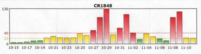
If we examine the ‘Ap’ Data for CR1848, covering October into November 1991 we can see the solar impact coincident with the formation of that storm.
It is important to note in all of our investigations that, although conditions may exist capable of causing a significant surface weather event, it does not follow that it always will – nature does not follow those rules. We can only assess an event and try to analyse the causal influences and estimate the likelihood of future events or occurrences of a similar nature arising.
As an incoming solar event or influence exerts what may most easily be visualised as a positive or negative ‘tidal’ pressure on the upper atmosphere structure, the result of that pressure will depend on the state of the atmosphere at that particular point in time. A northward or southward movement or tendency can be accelerated or delayed by the pressure applied; this will in turn influence the tracks of surface structures which may then reinforce the original distortion by dragging surface level air masses further north or south than would otherwise have been the case, thus exaggerating the intensity of those structures in a ‘positive feedback’ loop.
An illustration of this can be seen in the ‘Perfect Storm’ chart; the sharp negative influence of the drop in incoming solar activity, October 1991, will have increased the southward loop containing both the Canadian low pressure cell and the ex-hurricane cell. These will in turn have increased the western side southward cold flow together with the eastern side northward warm flow, exaggerating the blocking high, pushing the two lows together and intensifying the result. This effect may also have been involved in 1993 as the sharp up-spike in March of that year may well have intensified the ‘Super-storm’ of that month while the prolonged negative excursion over the latter half of 1993 undoubtedly gave rise to the wet and cold autumn and the noted severe winter of 1993/94.The upswing in 1994 represents a return to prevailing conditions from the conditions late 1993, rather than an impactive upswing.
To extrapolate further the observed tendencies of lower sunspot activity, together with lower coronal hole and solar wind activity, this does create the circumstance whereby an increased tendency towards more severe cold winters may be anticipated over coming decades; however to seriously assess long term behaviour we need to examine other factors such as the solar related increase in cosmic ray activity and the consequent increase in average cloud cover.
It is well established that reduced solar activity allows an increase in cosmic ray bombardment, the climatological impact of which is considered to cause an increase in cloud cover. The principal effect of this obviously being to increase the planetary albedo, or reflectivity, reducing the amount of solar radiation reaching the surface.

If, in conclusion, we now combine the reduction in sunspot activity associated with the expected ‘Maunder/Dalton Style’ decline over next few solar cycles; the anticipated decline in coronal hole / solar wind activity, plus the consequent cosmic ray/cloud cover behaviour, then we are inescapably left to conclude that a steady decline in surface climate and temperatures over the next few decades is almost beyond doubt.
C.D. 2017
